Note
Go to the end to download the full example code.
Using ExtensibleReactor to implement wall inertia#
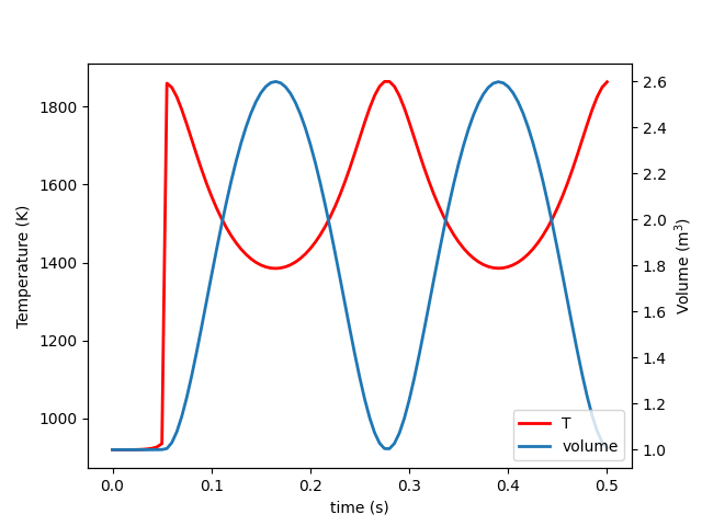
Solve an ignition problem where the normal reactor governing equations are extended with additional equations implemented in Python.
This demonstrates an approach for solving problems where Cantera’s built-in reactor
models are not sufficient for describing the system in question. Unlike the
custom.py example, in this example Cantera’s existing Reactor and
ReactorNet code is still used, with only the modifications to the standard equations
implemented in Python by extending the ExtensibleReactor class.
Wall objects in Cantera are normally massless, with the velocity either imposed or proportional to the pressure difference. Here, we simulate a wall where the acceleration is proportional to the pressure difference, and the velocity is determined by integrating the equation of motion. This requires adding a new variable to the reactor’s state vector which represents the wall velocity.
Requires: cantera >= 3.0, matplotlib >= 2.0

import cantera as ct
import numpy as np

class InertialWallReactor(ct.ExtensibleIdealGasReactor):
    def __init__(self, *args, neighbor, **kwargs):
        super().__init__(*args, **kwargs)
        self.v_wall = 0  # initial wall velocity
        self.k_wall = 1e-2  # proportionality constant, a_wall = k_wall * delta P
        self.neighbor = neighbor

    def after_initialize(self, t0):
        # The initialize function for the base Reactor class will have set
        # n_vars to already include the volume, internal energy, mass, and mass
        # fractions of all the species. Increase this by one to account for
        # the added variable of the wall velocity.
        self.n_vars += 1

        # The index for the new variable / equation, which is at the end of the
        # state vector
        self.i_wall = self.n_vars - 1

    def after_get_state(self, y):
        # This method is used to set the initial condition used by the ODE solver
        y[self.i_wall] = self.v_wall

    def after_update_state(self, y):
        # This method is used to set the state of the Reactor and Wall objects
        # based on the new values for the state vector provided by the ODE solver
        self.v_wall = y[self.i_wall]
        self.walls[0].velocity = self.v_wall

    def after_eval(self, t, LHS, RHS):
        # Calculate the time derivative for the additional equation
        a = self.k_wall * (self.thermo.P - self.neighbor.thermo.P)
        RHS[self.i_wall] = a

    def before_component_index(self, name):
        # Other components are handled by the method from the base Reactor class
        if name == 'v_wall':
            return self.i_wall

    def before_component_name(self, i):
        # Other components are handled by the method from the base Reactor class
        if i == self.i_wall:
            return 'v_wall'


gas = ct.Solution('h2o2.yaml')

# Initial condition
P = ct.one_atm
gas.TPY = 920, P, 'H2:1.0, O2:1.0, N2:3.76'

# Set up the reactor network
res = ct.Reservoir(gas)
r = InertialWallReactor(gas, neighbor=res)
w = ct.Wall(r, res)
net = ct.ReactorNet([r])

# Integrate the equations, keeping T(t) and Y(k,t)
states = ct.SolutionArray(gas, 1, extra={'t': [0.0], 'V': [r.volume]})
while net.time < 0.5:
    net.advance(net.time + 0.005)
    states.append(TPY=r.thermo.TPY, V=r.volume, t=net.time)

# Plot the results
try:
    import matplotlib.pyplot as plt
    L1 = plt.plot(states.t, states.T, color='r', label='T', lw=2)
    plt.xlabel('time (s)')
    plt.ylabel('Temperature (K)')
    plt.twinx()
    L2 = plt.plot(states.t, states.V, label='volume', lw=2)
    plt.ylabel('Volume (m$^3$)')
    plt.legend(L1+L2, [line.get_label() for line in L1+L2], loc='lower right')
    plt.show()
except ImportError:
    print('Matplotlib not found. Unable to plot results.')
Total running time of the script: (0 minutes 0.234 seconds)

