Note
Go to the end to download the full example code.
Shock-tube species profiles as a function of time#
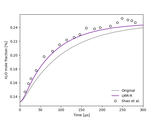
Simulate species profiles for a shock tube as a function of time, and observe the impact of incorporating the reduced-pressure linear mixture rule (LMR-R) in such calculations.
Here we predict the H2O mole fraction time profiles for a mixture of 1163 ppm H2O2/1330 ppm H2O/665 ppm O2/20% CO2/Ar following reflected shock waves (1196 K, 2.127 atm) and compare results against the experimental measurements of Shao et al. [1] Two models are compared in this example:
A 2023 model of H2 and NH3 chemistry published by Alzueta et al. [2]
An adapted version of this model that has applied the reduced-pressure linear mixture rule (LMR-R) and ab initio third-body efficiencies. [3]
References:
[1] J. Shao, R. Choudhary, D. F. Davidson, R. K. Hanson, Shock tube/laser absorption measurement of the rate constant of the reaction: H2O2+CO2 = 2OH+CO2, Proc. Combust. Inst. 39 (2023) 735 – 743.
[2] M. U. Alzueta, I. Salas, H. Hashemi, P. Glarborg, CO-assisted NH3 oxidation, Combust. Flame 257 (2023) 112438.
[3] P. J. Singal, J. Lee, L. Lei, R. L. Speth, M. P. Burke, Implementation of New Mixture Rules Has a Substantial Impact on Combustion Predictions for H2 and NH3, Proc. Combust. Inst. 40 (2024) 105779.
Requires: cantera >= 3.1, matplotlib
Run simulations with baseline and revised reaction mechanisms
for k, m in enumerate(models):
    X_H2O2 = 1163e-6
    X_H2O = 1330e-6
    X_O2 = 665e-6
    X_CO2= 0.2*(1-X_H2O2-X_H2O-X_O2)
    X_Ar = 1-X_CO2
    gas = ct.Solution(file, name=models[m])
    X = {'H2O2':X_H2O2, 'H2O':X_H2O, 'O2':X_O2, 'CO2':X_CO2, 'AR':X_Ar}
    gas.TPX = 1196, 2.127*ct.one_atm, X
    r = ct.Reactor(contents=gas,energy="on")
    reactorNetwork = ct.ReactorNet([r])
    timeHistory = ct.SolutionArray(gas, extra=['t'])
    estIgnitDelay = 1
    t = 0
    counter = 1
    while t < estIgnitDelay:
        t = reactorNetwork.step()
        if counter % 10 == 0:
            timeHistory.append(r.thermo.state, t=t)
        counter += 1

    results[m] = timeHistory
Plot the resulting species profiles and compare with the experimental data from Shao et al.
expData = {
    't': [12.3,20.3,26.4,39.6,58.5,79.2,96.1,113.8,131.6,145.7,161.2,181.6,195.3,219.9,
          237.2,248.6,262.4,272.2,280.9],
    'X_H2O': [1.47E-03,1.59E-03,1.66E-03,1.78E-03,1.98E-03,2.06E-03,2.15E-03,2.22E-03,
              2.26E-03,2.30E-03,2.39E-03,2.38E-03,2.40E-03,2.42E-03,2.47E-03,2.53E-03,
              2.51E-03,2.50E-03,2.47E-03]
}

fig, ax = plt.subplots()

for m, timeHistory in results.items():
    ax.plot(timeHistory.t*1e6, timeHistory('H2O').X*100, color=colors[m], label=m)

ax.plot(expData['t'], np.array(expData['X_H2O'])*100, 'o', fillstyle='none', color='k',
        label='Shao et al.')
ax.legend(frameon=False, loc='lower right')
ax.set_ylabel(r'$\rm H_2O$ mole fraction [%]')
ax.set_xlabel(r'Time [$\mathdefault{\mu s}$]')
ax.set_xlim([0,300])
plt.show()

Total running time of the script: (0 minutes 0.280 seconds)

