
Note
Go to the end to download the full example code.
Burner-stabilized flame with imposed temperature profile#
A burner-stabilized, premixed methane/air flat flame with multicomponent transport properties and a specified temperature profile.
Requires: cantera >= 3.0, matplotlib >= 2.0
from pathlib import Path
import numpy as np
import matplotlib.pyplot as plt
import cantera as ct
parameter values
p = ct.one_atm  # pressure
tburner = 373.7  # burner temperature
mdot = 0.04  # kg/m^2/s
comp = 'CH4:0.65, O2:1, N2:3.76'  # premixed gas composition

# The solution domain is chosen to be 1 cm
width = 0.01  # m

loglevel = 1  # amount of diagnostic output (0 to 5)
refine_grid = True  # 'True' to enable refinement
Create the gas object. This object will be used to evaluate all thermodynamic, kinetic, and transport properties
gas = ct.Solution('gri30.yaml')

# set its state to that of the unburned gas at the burner
gas.TPX = tburner, p, comp

# create the BurnerFlame object.
f = ct.BurnerFlame(gas=gas, width=width)

# set the mass flow rate at the burner
f.burner.mdot = mdot
Specify temperature vs. position data. For the purposes of this example, the data
is embedded directly. For more general use, the temperature profile should be stored
as a separate data file and read in, for example using np.genfromtxt.
zloc = np.array([
    0.        , 0.00015625, 0.00023437, 0.00039063, 0.00046875, 0.00050781,
    0.00054688, 0.000625  , 0.00066406, 0.00070312, 0.00074219, 0.00078125,
    0.00082031, 0.00085938, 0.00089844, 0.0009375 , 0.00101563, 0.00105469,
    0.00109375, 0.00113281, 0.00117187, 0.00121094, 0.00125   , 0.00128906,
    0.00132813, 0.00136719, 0.00140625, 0.00144531, 0.00148438, 0.00152344,
    0.0015625 , 0.00160156, 0.00164062, 0.00171875, 0.00175781, 0.00179688,
    0.00183594, 0.001875  , 0.00191406, 0.00195312, 0.00199219, 0.00203125,
    0.00207031, 0.00210938, 0.00214844, 0.0021875 , 0.00222656, 0.00226562,
    0.00230469, 0.00234375, 0.00238281, 0.00242187, 0.00246094, 0.0025    ,
    0.00257813, 0.00265625, 0.00273437, 0.0028125 , 0.00289062, 0.00296875,
    0.00304688, 0.003125  , 0.00328125, 0.0034375 , 0.00359375, 0.00375   ,
    0.00390625, 0.0087    , 0.01
])

tvalues = np.array([
     373.7      ,  465.4070428,  510.4311676,  599.5552837,  643.8342938,
     665.9335545,  688.0122338,  732.1284327,  754.1744755,  776.2170662,
     798.2588757,  820.3020011,  842.348001 ,  864.3979228,  886.4523159,
     908.5112198,  952.6396629,  974.7018199,  996.7515831, 1018.777651 ,
    1040.765863 , 1062.69948  , 1084.558639 , 1106.320078 , 1127.956918 ,
    1149.438472 , 1170.730129 , 1191.793309 , 1212.585506 , 1233.060477 ,
    1253.168589 , 1272.857384 , 1292.072391 , 1328.859767 , 1346.323998 ,
    1363.101361 , 1379.147594 , 1394.425274 , 1408.905834 , 1422.569115 ,
    1435.40408  , 1447.410648 , 1458.597668 , 1468.982722 , 1478.590978 ,
    1487.453914 , 1495.607879 , 1503.092709 , 1509.950449 , 1516.224147 ,
    1521.956853 , 1527.19079  , 1531.966722 , 1536.32348  , 1543.891739 ,
    1550.203579 , 1555.480771 , 1559.908135 , 1563.637879 , 1566.794144 ,
    1569.477867 , 1571.77099  , 1575.385829 , 1578.108169 , 1580.194856 ,
    1581.820666 , 1583.106578 , 1589.51315  , 1589.578955
])

zloc /= max(zloc)

# set the temperature profile to the values read in
f.flame.set_fixed_temp_profile(zloc, tvalues)
show the initial estimate for the solution
f.show()

# don't solve the energy equation
f.energy_enabled = False

# first solve the flame with mixture-averaged transport properties
f.transport_model = 'mixture-averaged'
f.set_refine_criteria(ratio=3.0, slope=0.3, curve=1)

f.solve(loglevel, refine_grid)

if "native" in ct.hdf_support():
    output = Path() / "flame_fixed_T.h5"
else:
    output = Path() / "flame_fixed_T.yaml"
output.unlink(missing_ok=True)

f.save(output, name="mix", description="solution with mixture-averaged transport")

print('\n\n switching to multicomponent transport...\n\n')
f.transport_model = 'multicomponent'

f.set_refine_criteria(ratio=3.0, slope=0.1, curve=0.2)
f.solve(loglevel, refine_grid)
f.save(output, name="multi", description="solution with multicomponent transport")

# write the velocity, temperature, density, and mole fractions to a CSV file
f.save('flame_fixed_T.csv', basis="mole", overwrite=True)
f.show_stats()
>>>>>>>>>>>>>>>>>>>>>>>>>>>>>>>>> burner <<<<<<<<<<<<<<<<<<<<<<<<<<<<<<<<<

    Mass Flux:         0.04 kg/m^2/s
    Temperature:      373.7 K
    Mass Fractions:
                      O2      0.2166
                     CH4     0.07057
                      N2      0.7129


>>>>>>>>>>>>>>>>>>>>>>>>>>>>>>>>> flame <<<<<<<<<<<<<<<<<<<<<<<<<<<<<<<<<

    Pressure:   1.013e+05 Pa

-------------------------------------------------------------------------------
          z    velocity  spread_rate           T      lambda      eField
-------------------------------------------------------------------------------
          0     0.04491           0       373.7           0           0
      0.001      0.1562           0        1240           0           0
      0.002      0.2674           0        2107           0           0
      0.003      0.2674           0        2107           0           0
      0.005      0.2674           0        2107           0           0
      0.007      0.2674           0        2107           0           0
       0.01      0.2674           0        2107           0           0

-------------------------------------------------------------------------------
          z          Uo          H2           H           O          O2
-------------------------------------------------------------------------------
          0           0           0           0           0      0.2166
      0.001           0    0.001694   1.324e-05   1.187e-06      0.1083
      0.002           0    0.003388   2.649e-05   2.375e-06   8.549e-06
      0.003           0    0.003388   2.649e-05   2.375e-06   8.549e-06
      0.005           0    0.003388   2.649e-05   2.375e-06   8.549e-06
      0.007           0    0.003388   2.649e-05   2.375e-06   8.549e-06
       0.01           0    0.003388   2.649e-05   2.375e-06   8.549e-06

-------------------------------------------------------------------------------
          z          OH         H2O         HO2        H2O2           C
-------------------------------------------------------------------------------
          0           0           0           0           0           0
      0.001   0.0001135     0.06393    1.61e-09   8.313e-10   7.198e-17
      0.002    0.000227      0.1279    3.22e-09   1.663e-09    1.44e-16
      0.003    0.000227      0.1279    3.22e-09   1.663e-09    1.44e-16
      0.005    0.000227      0.1279    3.22e-09   1.663e-09    1.44e-16
      0.007    0.000227      0.1279    3.22e-09   1.663e-09    1.44e-16
       0.01    0.000227      0.1279    3.22e-09   1.663e-09    1.44e-16

-------------------------------------------------------------------------------
          z          CH         CH2      CH2(S)         CH3         CH4
-------------------------------------------------------------------------------
          0           0           0           0           0     0.07057
      0.001   5.988e-17   1.245e-15   6.747e-17   6.201e-14     0.03529
      0.002   1.198e-16    2.49e-15   1.349e-16    1.24e-13   4.373e-13
      0.003   1.198e-16    2.49e-15   1.349e-16    1.24e-13   4.373e-13
      0.005   1.198e-16    2.49e-15   1.349e-16    1.24e-13   4.373e-13
      0.007   1.198e-16    2.49e-15   1.349e-16    1.24e-13   4.373e-13
       0.01   1.198e-16    2.49e-15   1.349e-16    1.24e-13   4.373e-13

-------------------------------------------------------------------------------
          z          CO         CO2         HCO        CH2O       CH2OH
-------------------------------------------------------------------------------
          0           0           0           0           0           0
      0.001     0.03328     0.04451   6.693e-09   6.348e-10   5.328e-15
      0.002     0.06656     0.08903   1.339e-08    1.27e-09   1.066e-14
      0.003     0.06656     0.08903   1.339e-08    1.27e-09   1.066e-14
      0.005     0.06656     0.08903   1.339e-08    1.27e-09   1.066e-14
      0.007     0.06656     0.08903   1.339e-08    1.27e-09   1.066e-14
       0.01     0.06656     0.08903   1.339e-08    1.27e-09   1.066e-14

-------------------------------------------------------------------------------
          z        CH3O       CH3OH         C2H        C2H2        C2H3
-------------------------------------------------------------------------------
          0           0           0           0           0           0
      0.001   7.758e-17   2.904e-15     1.7e-20    4.29e-17   9.646e-22
      0.002   1.552e-16   5.808e-15     3.4e-20   8.579e-17   1.929e-21
      0.003   1.552e-16   5.808e-15     3.4e-20   8.579e-17   1.929e-21
      0.005   1.552e-16   5.808e-15     3.4e-20   8.579e-17   1.929e-21
      0.007   1.552e-16   5.808e-15     3.4e-20   8.579e-17   1.929e-21
       0.01   1.552e-16   5.808e-15     3.4e-20   8.579e-17   1.929e-21

-------------------------------------------------------------------------------
          z        C2H4        C2H5        C2H6        HCCO       CH2CO
-------------------------------------------------------------------------------
          0           0           0           0           0           0
      0.001    7.73e-21   2.486e-25   1.202e-25   5.191e-17   4.844e-16
      0.002   1.546e-20   4.971e-25   2.404e-25   1.038e-16   9.688e-16
      0.003   1.546e-20   4.971e-25   2.404e-25   1.038e-16   9.688e-16
      0.005   1.546e-20   4.971e-25   2.404e-25   1.038e-16   9.688e-16
      0.007   1.546e-20   4.971e-25   2.404e-25   1.038e-16   9.688e-16
       0.01   1.546e-20   4.971e-25   2.404e-25   1.038e-16   9.688e-16

-------------------------------------------------------------------------------
          z       HCCOH           N          NH         NH2         NH3
-------------------------------------------------------------------------------
          0           0           0           0           0           0
      0.001   3.173e-19   8.648e-10   7.756e-10   1.917e-09    4.21e-08
      0.002   6.347e-19    1.73e-09   1.551e-09   3.834e-09   8.419e-08
      0.003   6.347e-19    1.73e-09   1.551e-09   3.834e-09   8.419e-08
      0.005   6.347e-19    1.73e-09   1.551e-09   3.834e-09   8.419e-08
      0.007   6.347e-19    1.73e-09   1.551e-09   3.834e-09   8.419e-08
       0.01   6.347e-19    1.73e-09   1.551e-09   3.834e-09   8.419e-08

-------------------------------------------------------------------------------
          z         NNH          NO         NO2         N2O         HNO
-------------------------------------------------------------------------------
          0           0           0           0           0           0
      0.001    6.43e-10   3.093e-05   3.977e-10    2.33e-09   1.888e-09
      0.002   1.286e-09   6.186e-05   7.954e-10   4.661e-09   3.777e-09
      0.003   1.286e-09   6.186e-05   7.954e-10   4.661e-09   3.777e-09
      0.005   1.286e-09   6.186e-05   7.954e-10   4.661e-09   3.777e-09
      0.007   1.286e-09   6.186e-05   7.954e-10   4.661e-09   3.777e-09
       0.01   1.286e-09   6.186e-05   7.954e-10   4.661e-09   3.777e-09

-------------------------------------------------------------------------------
          z          CN         HCN        H2CN        HCNN        HCNO
-------------------------------------------------------------------------------
          0           0           0           0           0           0
      0.001   1.088e-12   2.824e-09   2.049e-15   1.011e-19    8.02e-16
      0.002   2.175e-12   5.648e-09   4.098e-15   2.023e-19   1.604e-15
      0.003   2.175e-12   5.648e-09   4.098e-15   2.023e-19   1.604e-15
      0.005   2.175e-12   5.648e-09   4.098e-15   2.023e-19   1.604e-15
      0.007   2.175e-12   5.648e-09   4.098e-15   2.023e-19   1.604e-15
       0.01   2.175e-12   5.648e-09   4.098e-15   2.023e-19   1.604e-15

-------------------------------------------------------------------------------
          z        HOCN        HNCO         NCO          N2          AR
-------------------------------------------------------------------------------
          0           0           0           0      0.7129           0
      0.001   1.588e-11   7.375e-09   3.844e-11      0.7129           0
      0.002   3.176e-11   1.475e-08   7.688e-11      0.7128           0
      0.003   3.176e-11   1.475e-08   7.688e-11      0.7128           0
      0.005   3.176e-11   1.475e-08   7.688e-11      0.7128           0
      0.007   3.176e-11   1.475e-08   7.688e-11      0.7128           0
       0.01   3.176e-11   1.475e-08   7.688e-11      0.7128           0

-------------------------------------------------------------------------------
          z        C3H7        C3H8      CH2CHO      CH3CHO
-------------------------------------------------------------------------------
          0           0           0           0           0
      0.001   2.615e-37   1.186e-37   5.824e-21   7.352e-21
      0.002    5.23e-37   2.373e-37   1.165e-20    1.47e-20
      0.003    5.23e-37   2.373e-37   1.165e-20    1.47e-20
      0.005    5.23e-37   2.373e-37   1.165e-20    1.47e-20
      0.007    5.23e-37   2.373e-37   1.165e-20    1.47e-20
       0.01    5.23e-37   2.373e-37   1.165e-20    1.47e-20


>>>>>>>>>>>>>>>>>>>>>>>>>>>>>>>>> outlet <<<<<<<<<<<<<<<<<<<<<<<<<<<<<<<<<


-------------------------------------------------------------------------------
          z
-------------------------------------------------------------------------------
          0

..............................................................................

Attempt Newton solution of steady-state problem.
Newton steady-state solve failed.

Attempt 10 timesteps.
Final timestep info: dt= 8.009e-06  log(ss)= 1.656

Attempt Newton solution of steady-state problem.
Newton steady-state solve failed.

Attempt 10 timesteps.
Final timestep info: dt= 0.0001368  log(ss)= 1.471

Attempt Newton solution of steady-state problem.
Newton steady-state solve failed.

Attempt 10 timesteps.
Final timestep info: dt= 0.002338   log(ss)= -0.07942

Attempt Newton solution of steady-state problem.
Newton steady-state solve succeeded.

Problem solved on [7] point grid(s).

..............................................................................
##############################################################################
Refining grid in flame.
    New points inserted after grid points 0 1 2 3
    to resolve C2H2 C2H3 C2H4 C2H5 C2H6 C3H8 CH2 CH2CHO CH2CO CH2O CH2OH CH3 CH3CHO CH3O CH3OH CH4 CO CO2 H H2 H2O H2O2 HCCO HCCOH HCN HCO HNCO HO2 NO NO2 O O2 OH
##############################################################################

..............................................................................

Attempt Newton solution of steady-state problem.
Newton steady-state solve succeeded.

Problem solved on [11] point grid(s).

..............................................................................
##############################################################################
Refining grid in flame.
    New points inserted after grid points 0 1 2 3 4 5 6
    to resolve C2H2 C2H3 C2H4 C2H5 C2H6 C3H8 CH2 CH2CHO CH2CO CH2O CH2OH CH3 CH3CHO CH3O CH3OH H H2O2 HCCO HCCOH HCO HO2 NO2 O OH
##############################################################################

..............................................................................

Attempt Newton solution of steady-state problem.
Newton steady-state solve succeeded.

Problem solved on [18] point grid(s).

..............................................................................
##############################################################################
Refining grid in flame.
    New points inserted after grid points 3 5 6 7 8 9 12
    to resolve C2H3 C2H5 C3H8 CH2 CH2CHO CH3 CH3CHO H2O2 HCCO HCO O OH
##############################################################################

..............................................................................

Attempt Newton solution of steady-state problem.
Newton steady-state solve succeeded.

Problem solved on [25] point grid(s).

..............................................................................
no new points needed in flame


 switching to multicomponent transport...


..............................................................................

Attempt Newton solution of steady-state problem.
Newton steady-state solve succeeded.

Problem solved on [25] point grid(s).

..............................................................................
##############################################################################
Refining grid in flame.
    New points inserted after grid points 0 1 2 3 4 5 6 7 8 9 10 11 12 13 14 15 16 17 18 19 20 21 22
    to resolve C2H2 C2H3 C2H4 C2H5 C2H6 C3H8 CH2 CH2CHO CH2CO CH2O CH2OH CH3 CH3CHO CH3O CH3OH CH4 CO H H2 H2O H2O2 HCCO HCCOH HCO HO2 N2 NO2 O O2 OH
##############################################################################

..............................................................................

Attempt Newton solution of steady-state problem.
Newton steady-state solve succeeded.

Problem solved on [48] point grid(s).

..............................................................................
##############################################################################
Refining grid in flame.
    New points inserted after grid points 3 4 5 10 11 13 14 23 24 25 26 32 33 34 35 36 40 42 46
    to resolve C2H3 C2H4 C2H5 C3H8 CH2 CH2CHO CH2CO CH3CHO CH3O H H2O2 HCCO HCO HO2 O OH point 46
##############################################################################

..............................................................................

Attempt Newton solution of steady-state problem.
Newton steady-state solve succeeded.

Problem solved on [67] point grid(s).

..............................................................................
no new points needed in flame

Statistics:

 Grid   Timesteps  Functions      Time  Jacobians      Time
    9          30        476    0.2701         21    2.2445
   13           0         44    0.0366          2    0.3763
   20           0         12    0.0296          1    0.3148
   27           0          4    0.0024          1    0.4120
   27           0          2    0.0606          1    0.2762
   50           0          4    0.2501          1    0.4899
   69           0          4    0.3542          1    0.4390
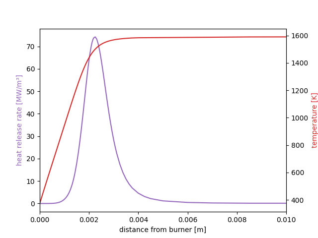
Temperature and Heat Release Rate#
fig, ax1 = plt.subplots()

ax1.plot(f.grid, f.heat_release_rate / 1e6, color='C4')
ax1.set_ylabel('heat release rate [MW/m³]', color='C4')
ax1.set_xlim(0, 0.01)
ax1.set(xlabel='distance from burner [m]')

ax2 = ax1.twinx()
ax2.plot(f.grid, f.T, color='C3')
ax2.set_ylabel('temperature [K]', color='C3')
plt.show()
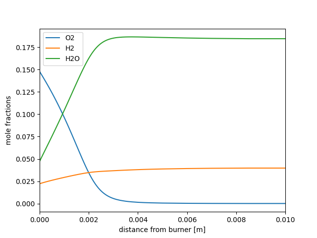
Major Species Profiles#
fig, ax = plt.subplots()
major = ('O2', 'H2', 'H2O')
states = f.to_array()
ax.plot(states.grid, states(*major).X, label=major)
ax.set(xlabel='distance from burner [m]', ylabel='mole fractions')
ax.set_xlim(0, 0.01)
ax.legend()
plt.show()
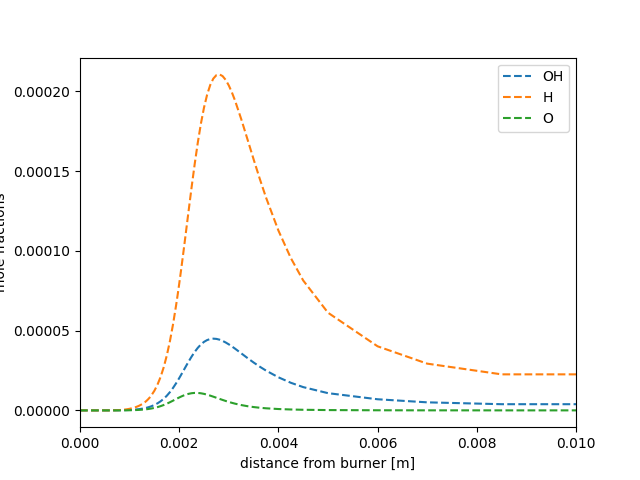
Minor Species Profiles#
fig, ax = plt.subplots()
minor = ('OH', 'H', 'O')

ax.plot(states.grid, states(*minor).X, label=minor, linestyle='--')
ax.set(xlabel='distance from burner [m]', ylabel='mole fractions', )
ax.set_xlim(0, 0.01)
ax.legend()
plt.show()
Total running time of the script: (0 minutes 2.552 seconds)